Getting started
Authors: Alan Murphy, Brian Schilder, and Nathan Skene
Authors: Alan Murphy, Brian Schilder, and Nathan Skene
Updated: Mar-20-2026
Source: Updated: Mar-20-2026
vignettes/EWCE.Rmd
EWCE.RmdIntroduction
The EWCE R package is designed to facilitate expression
weighted cell type enrichment analysis as described in our Frontiers
in Neuroscience paper1.
EWCE can be applied to any gene list.
Using EWCE essentially involves two steps:
- Prepare a single-cell reference; i.e. CellTypeDataset (CTD).
Alternatively, you can use one of the pre-generated CTDs we provide via
the package
ewceData(which comes withEWCE).
- Run cell type enrichment on a gene list using the
bootstrap_enrichment_testfunction.
NOTE: This documentation is for the development
version of EWCE. See Bioconductor
for documentation on the current release version.
Setup
## Loading required package: RNOmni## Registered S3 method overwritten by 'bit64':
## method from
## print.bitstring toolsRun cell-type enrichment tests
1. Prepare input data
CellTypeDataset
Load a CTD previously generated from mouse cortex and hypothalamus single-cell RNA-seq data (from the Karolinska Institute).
CTD levels
Each level of a CTD corresponds to increasingly refined
cell-type/-subtype annotations. For example, in the CTD
ewceData::ctd() level 1 includes the cell-type
“interneurons”, while level 2 breaks these this group into 16 different
interneuron subtypes (“Int…”).
ctd <- ewceData::ctd()## see ?ewceData and browseVignettes('ewceData') for documentation## Error while performing HEAD request.
## Proceeding without cache information.## loading from cache## Error while performing HEAD request.
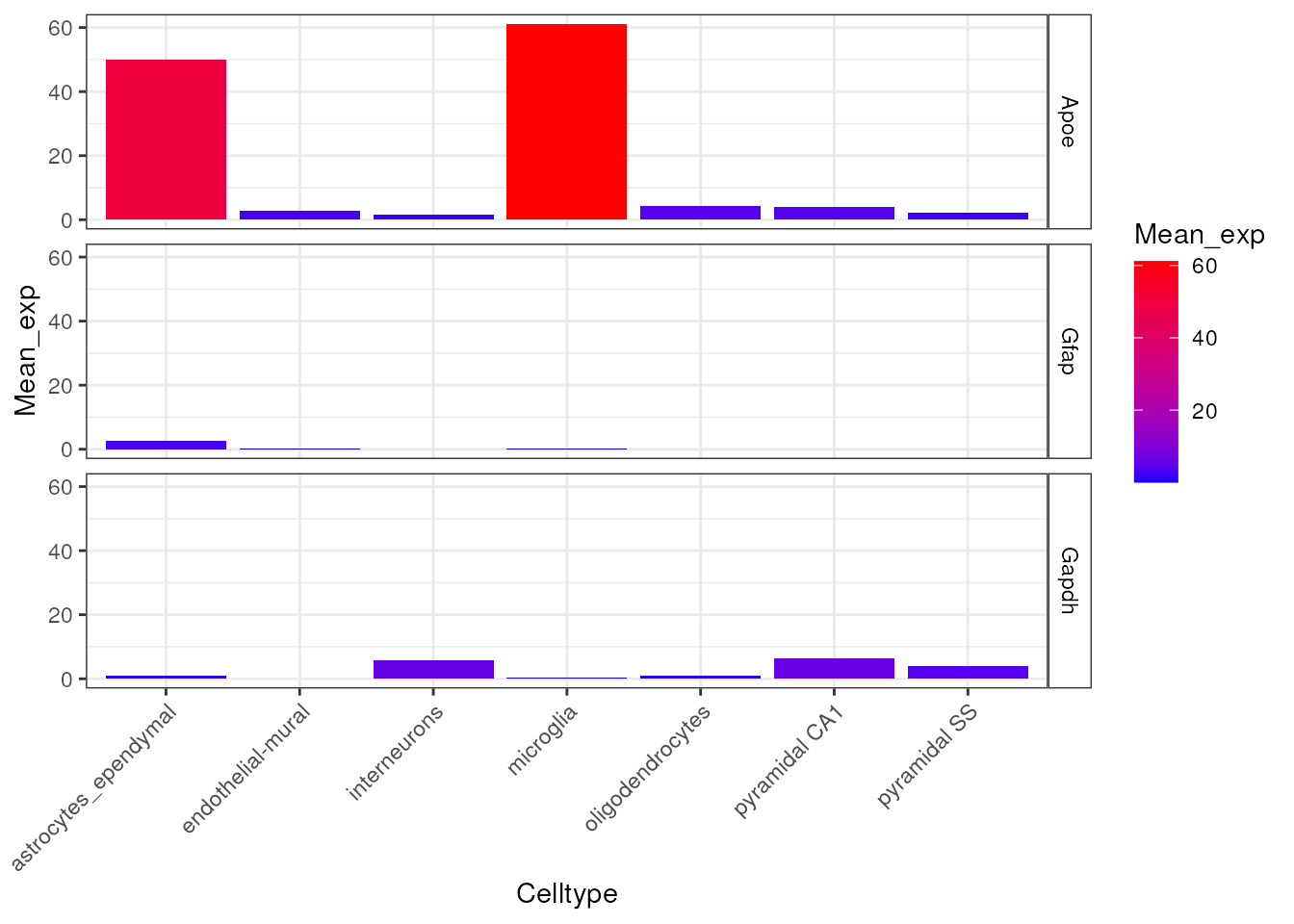
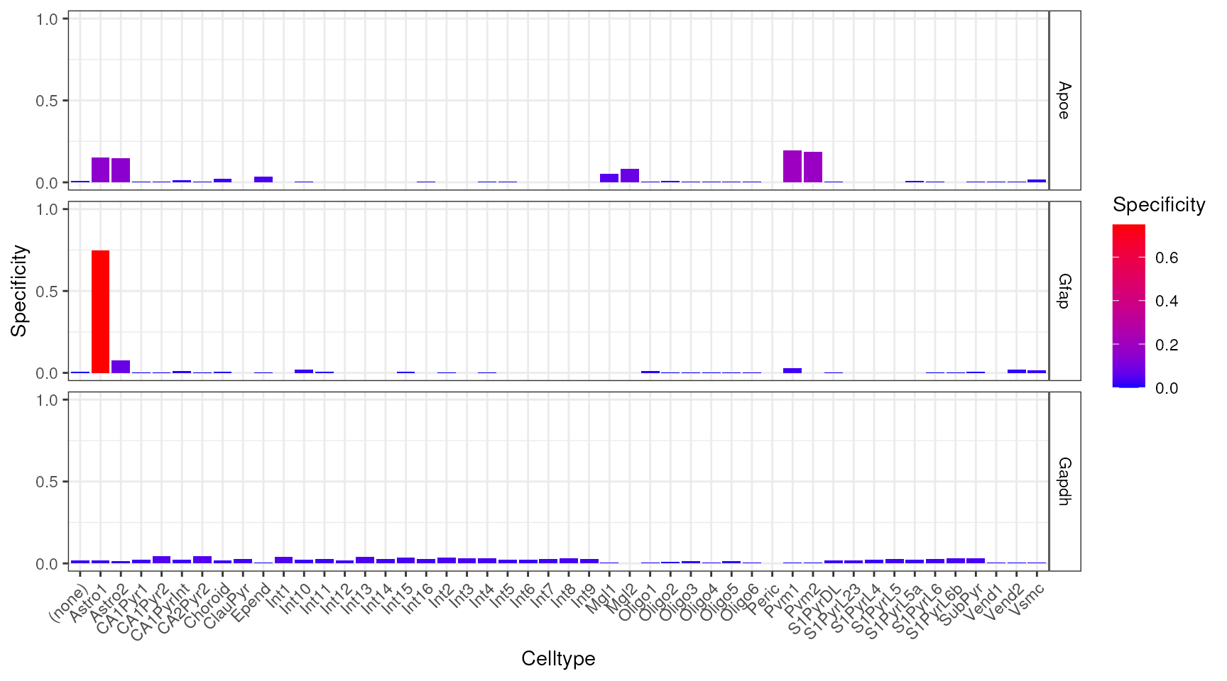
## Proceeding without cache information.Plot CTD mean_exp
Plot the expression of four markers genes across all cell types in the CTD.
plt_exp <- EWCE::plot_ctd(ctd = ctd,
                        level = 1,
                        genes = c("Apoe","Gfap","Gapdh"),
                        metric = "mean_exp")
plt_spec <- EWCE::plot_ctd(ctd = ctd,
                         level = 2,
                         genes = c("Apoe","Gfap","Gapdh"),
                         metric = "specificity")
Gene list
Gene lists input into EWCE can comes from any source (e.g. GWAS, candidate genes, pathways).
Here, we provide an example gene list of Alzheimer’s disease-related nominated from a GWAS.
hits <- ewceData::example_genelist()## see ?ewceData and browseVignettes('ewceData') for documentation## loading from cache
print(hits)## [1] "APOE" "BIN1" "CLU" "ABCA7" "CR1" "PICALM"
## [7] "MS4A6A" "CD33" "MS4A4E" "CD2AP" "EOGA1" "INPP5D"
## [13] "MEF2C" "HLA-DRB5" "ZCWPW1" "NME8" "PTK2B" "CELF1"
## [19] "SORL1" "FERMT2" "SLC24A4" "CASS4"2. Run cell type enrichment tests
We now run the cell type enrichment tests on the gene list. Since the
CTD is from mouse data (and is annotated using mouse genes) we specify
the argument sctSpecies="mouse".
bootstrap_enrichment_test will automaticlaly convert the
mouse genes to human genes.
Since the gene list came from GWAS in humans, we set
genelistSpecies="human".
Note: We set the seed at the top of this vignette to ensure reproducibility in the bootstrap sampling function.
Hyperparameters
Note: We use 100 repetitions here for the purposes of a
quick example, but in practice you would want to use
reps=10000 for publishable results.
Parallelisation
You can now speed up the bootstrapping process by parallelising
across multiple cores with the parameter no_cores
(=1 by default).
reps <- 100
annotLevel <- 1
full_results <- EWCE::bootstrap_enrichment_test(sct_data = ctd,
                                                sctSpecies = "mouse",
                                                genelistSpecies = "human",
                                                hits = hits,
                                                reps = reps,
                                                annotLevel = annotLevel)
## 1 core(s) assigned as workers (3 reserved).## Generating gene background for mouse x human ==> human## Gathering ortholog reports.## Retrieving all genes using: homologene.## Retrieving all organisms available in homologene.## Mapping species name: human## Common name mapping found for human## 1 organism identified from search: 9606## Using cached file: /github/home/.cache/R/orthogene/all_genes-9606-homologene.csv.gz## Returning all 19,129 genes from human.## Retrieving all genes using: homologene.## Retrieving all organisms available in homologene.## Mapping species name: mouse## Common name mapping found for mouse## 1 organism identified from search: 10090## Using cached file: /github/home/.cache/R/orthogene/all_genes-10090-homologene.csv.gz## Returning all 21,207 genes from mouse.## --
## --## Preparing gene_df.## data.table format detected.## Extracting genes from Gene.Symbol.## 21,207 genes extracted.## Converting mouse ==> human orthologs using: homologene## Retrieving all organisms available in homologene.## Mapping species name: mouse## Common name mapping found for mouse## 1 organism identified from search: 10090## Retrieving all organisms available in homologene.## Mapping species name: human## Common name mapping found for human## 1 organism identified from search: 9606## Checking for genes without orthologs in human.## Extracting genes from input_gene.## 17,355 genes extracted.## Extracting genes from ortholog_gene.## 17,355 genes extracted.## Checking for genes without 1:1 orthologs.## Dropping 131 genes that have multiple input_gene per ortholog_gene (many:1).## Dropping 498 genes that have multiple ortholog_gene per input_gene (1:many).## Filtering gene_df with gene_map## Adding input_gene col to gene_df.## Adding ortholog_gene col to gene_df.##
## =========== REPORT SUMMARY ===========## Total genes dropped after convert_orthologs :
## 4,725 / 21,207 (22%)## Total genes remaining after convert_orthologs :
## 16,482 / 21,207 (78%)## --##
## =========== REPORT SUMMARY ===========## 16,482 / 21,207 (77.72%) target_species genes remain after ortholog conversion.## 16,482 / 19,129 (86.16%) reference_species genes remain after ortholog conversion.## Gathering ortholog reports.## Retrieving all genes using: homologene.## Retrieving all organisms available in homologene.## Mapping species name: human## Common name mapping found for human## 1 organism identified from search: 9606## Using cached file: /github/home/.cache/R/orthogene/all_genes-9606-homologene.csv.gz## Returning all 19,129 genes from human.## Retrieving all genes using: homologene.## Retrieving all organisms available in homologene.## Mapping species name: human## Common name mapping found for human## 1 organism identified from search: 9606## Using cached file: /github/home/.cache/R/orthogene/all_genes-9606-homologene.csv.gz## Returning all 19,129 genes from human.## --##
## =========== REPORT SUMMARY ===========## 19,129 / 19,129 (100%) target_species genes remain after ortholog conversion.## 19,129 / 19,129 (100%) reference_species genes remain after ortholog conversion.## 16,482 intersect background genes used.## Standardising CellTypeDataset## Checking gene list inputs.## Running without gene size control.## 17 hit gene(s) remain after filtering.## Computing gene scores.## Using previously sampled genes.## Computing gene counts.## Testing for enrichment in 7 cell types...## Sorting results by p-value.## Computing BH-corrected q-values.## 1 significant cell type enrichment results @ q<0.05 :## CellType annotLevel p fold_change sd_from_mean q
## 1 microglia 1 0 1.965915 3.938119 0The main table of results is stored in
full_results$results.
In this case, microglia were the only cell type that was significantly enriched in the Alzheimer’s disease gene list.
knitr::kable(full_results$results)| CellType | annotLevel | p | fold_change | sd_from_mean | q | |
|---|---|---|---|---|---|---|
| microglia | microglia | 1 | 0.00 | 1.9659148 | 3.9381188 | 0.000 |
| astrocytes_ependymal | astrocytes_ependymal | 1 | 0.13 | 1.2624889 | 1.1553910 | 0.455 |
| pyramidal_SS | pyramidal_SS | 1 | 0.80 | 0.8699242 | -0.8226268 | 1.000 |
| oligodendrocytes | oligodendrocytes | 1 | 0.87 | 0.7631149 | -1.0861761 | 1.000 |
| pyramidal_CA1 | pyramidal_CA1 | 1 | 0.89 | 0.8202496 | -1.1738063 | 1.000 |
| endothelial_mural | endothelial_mural | 1 | 0.90 | 0.7674534 | -1.1811797 | 1.000 |
| interneurons | interneurons | 1 | 1.00 | 0.4012954 | -3.4703413 | 1.000 |
The results can be visualised using another function, which shows for each cell type, the number of standard deviations from the mean the level of expression was found to be in the target gene list, relative to the bootstrapped mean.
The dendrogram at the top shows how the cell types are hierarchically clustered by transcriptional similarity.
plot_list <- EWCE::ewce_plot(total_res = full_results$results,
                           mtc_method = "BH",
                           ctd = ctd)
print(plot_list$withDendro)
## NULLDocker
ewce is now available via DockerHub as a containerised environment with Rstudio and all necessary dependencies pre-installed.
Method 1: via Docker
First, install Docker if you have not already.
Create an image of the Docker container in command line:
docker pull neurogenomicslab/ewceOnce the image has been created, you can launch it with:
docker run \
  -d \
  -e ROOT=true \
  -e PASSWORD=bioc \
  -v ~/Desktop:/Desktop \
  -v /Volumes:/Volumes \
  -p 8787:8787 \
neurogenomicslab/ewce- The
-densures the container will run in “detached” mode, which means it will persist even after you’ve closed your command line session.
- Optionally, you can also install the Docker Desktop
to easily manage your containers.
- You can set the password to whatever you like by changing the
-e PASSWORD=...flag.
- The username will be “rstudio” by default.
Method 2: via Singularity
If you are using a system that does not allow Docker (as is the case for many institutional computing clusters), you can instead install Docker images via Singularity.
singularity pull docker://neurogenomicslab/ewceUsage
Finally, launch the containerised Rstudio by entering the following URL in any web browser: http://localhost:8787/
Login using the credentials set during the Installation steps.
Session Info
utils::sessionInfo()## R Under development (unstable) (2026-03-15 r89629)
## Platform: x86_64-pc-linux-gnu
## Running under: Ubuntu 24.04.4 LTS
##
## Matrix products: default
## BLAS: /usr/lib/x86_64-linux-gnu/openblas-pthread/libblas.so.3
## LAPACK: /usr/lib/x86_64-linux-gnu/openblas-pthread/libopenblasp-r0.3.26.so; LAPACK version 3.12.0
##
## locale:
## [1] LC_CTYPE=en_US.UTF-8 LC_NUMERIC=C
## [3] LC_TIME=en_US.UTF-8 LC_COLLATE=en_US.UTF-8
## [5] LC_MONETARY=en_US.UTF-8 LC_MESSAGES=en_US.UTF-8
## [7] LC_PAPER=en_US.UTF-8 LC_NAME=C
## [9] LC_ADDRESS=C LC_TELEPHONE=C
## [11] LC_MEASUREMENT=en_US.UTF-8 LC_IDENTIFICATION=C
##
## time zone: UTC
## tzcode source: system (glibc)
##
## attached base packages:
## [1] stats graphics grDevices utils datasets methods base
##
## other attached packages:
## [1] ewceData_1.19.0 ExperimentHub_3.1.0 AnnotationHub_4.1.0
## [4] BiocFileCache_3.1.0 dbplyr_2.5.2 BiocGenerics_0.57.0
## [7] generics_0.1.4 EWCE_1.19.1 RNOmni_1.0.1.2
## [10] BiocStyle_2.39.0
##
## loaded via a namespace (and not attached):
## [1] RColorBrewer_1.1-3 jsonlite_2.0.0
## [3] magrittr_2.0.4 farver_2.1.2
## [5] rmarkdown_2.30 fs_1.6.7
## [7] ragg_1.5.1 vctrs_0.7.1
## [9] memoise_2.0.1 ggtree_4.1.1
## [11] rstatix_0.7.3 htmltools_0.5.9
## [13] S4Arrays_1.11.1 curl_7.0.0
## [15] broom_1.0.12 SparseArray_1.11.11
## [17] Formula_1.2-5 gridGraphics_0.5-1
## [19] sass_0.4.10 bslib_0.10.0
## [21] htmlwidgets_1.6.4 desc_1.4.3
## [23] plyr_1.8.9 HGNChelper_0.8.15
## [25] httr2_1.2.2 plotly_4.12.0
## [27] cachem_1.1.0 lifecycle_1.0.5
## [29] pkgconfig_2.0.3 Matrix_1.7-4
## [31] R6_2.6.1 fastmap_1.2.0
## [33] MatrixGenerics_1.23.0 digest_0.6.39
## [35] aplot_0.2.9 patchwork_1.3.2
## [37] AnnotationDbi_1.73.0 S4Vectors_0.49.0
## [39] textshaping_1.0.5 GenomicRanges_1.63.1
## [41] RSQLite_2.4.6 ggpubr_0.6.3
## [43] labeling_0.4.3 filelock_1.0.3
## [45] httr_1.4.8 abind_1.4-8
## [47] compiler_4.6.0 withr_3.0.2
## [49] bit64_4.6.0-1 fontquiver_0.2.1
## [51] S7_0.2.1 backports_1.5.0
## [53] BiocParallel_1.45.0 orthogene_1.17.2
## [55] carData_3.0-6 DBI_1.3.0
## [57] homologene_1.4.68.19.3.27 R.utils_2.13.0
## [59] ggsignif_0.6.4 MASS_7.3-65
## [61] rappdirs_0.3.4 DelayedArray_0.37.0
## [63] tools_4.6.0 splitstackshape_1.4.8
## [65] otel_0.2.0 ape_5.8-1
## [67] R.oo_1.27.1 glue_1.8.0
## [69] nlme_3.1-168 grid_4.6.0
## [71] reshape2_1.4.5 gtable_0.3.6
## [73] R.methodsS3_1.8.2 tidyr_1.3.2
## [75] data.table_1.18.2.1 car_3.1-5
## [77] XVector_0.51.0 stringr_1.6.0
## [79] BiocVersion_3.23.1 pillar_1.11.1
## [81] yulab.utils_0.2.4 babelgene_22.9
## [83] limma_3.67.0 dplyr_1.2.0
## [85] treeio_1.35.0 lattice_0.22-9
## [87] bit_4.6.0 tidyselect_1.2.1
## [89] fontLiberation_0.1.0 SingleCellExperiment_1.33.1
## [91] Biostrings_2.79.5 knitr_1.51
## [93] fontBitstreamVera_0.1.1 bookdown_0.46
## [95] IRanges_2.45.0 Seqinfo_1.1.0
## [97] SummarizedExperiment_1.41.1 stats4_4.6.0
## [99] xfun_0.56 Biobase_2.71.0
## [101] statmod_1.5.1 matrixStats_1.5.0
## [103] stringi_1.8.7 lazyeval_0.2.2
## [105] ggfun_0.2.0 yaml_2.3.12
## [107] codetools_0.2-20 evaluate_1.0.5
## [109] gdtools_0.5.0 tibble_3.3.1
## [111] BiocManager_1.30.27 ggplotify_0.1.3
## [113] cli_3.6.5 systemfonts_1.3.2
## [115] jquerylib_0.1.4 Rcpp_1.1.1
## [117] gprofiler2_0.2.4 png_0.1-9
## [119] parallel_4.6.0 pkgdown_2.2.0
## [121] ggplot2_4.0.2 blob_1.3.0
## [123] viridisLite_0.4.3 tidytree_0.4.7
## [125] ggiraph_0.9.6 scales_1.4.0
## [127] purrr_1.2.1 crayon_1.5.3
## [129] rlang_1.1.7 KEGGREST_1.51.1